On this Page
...
- Profiling: Use Profile Snap from ML Analytics Snap Pack to get statistics of this dataset.
- Data Preparation: Perform data preparation on this dataset using Snaps in ML Data Preparation Snap Pack.
- AutoML: Use AutoML Snap from ML Core Snap Pack to build models and pick the one with the best performance.
- Cross Validation: Use Cross Validator (Classification) Snap from ML Core Snap Pack to perform 10-fold cross validation on various Machine Learning algorithms. The result will let us know the accuracy of each algorithm in the success rate prediction.
We are going to build 4 pipelines5 Pipelines: Profiling, Data Preparation, Data Modelling and 2 pipelines Pipelines for Cross Validation with various algorithms. Each of these pipelines Pipelines is described in the Pipelines section below.
Pipelines
Profiling
In order to get useful statistics, we need to transform the data a little bit.

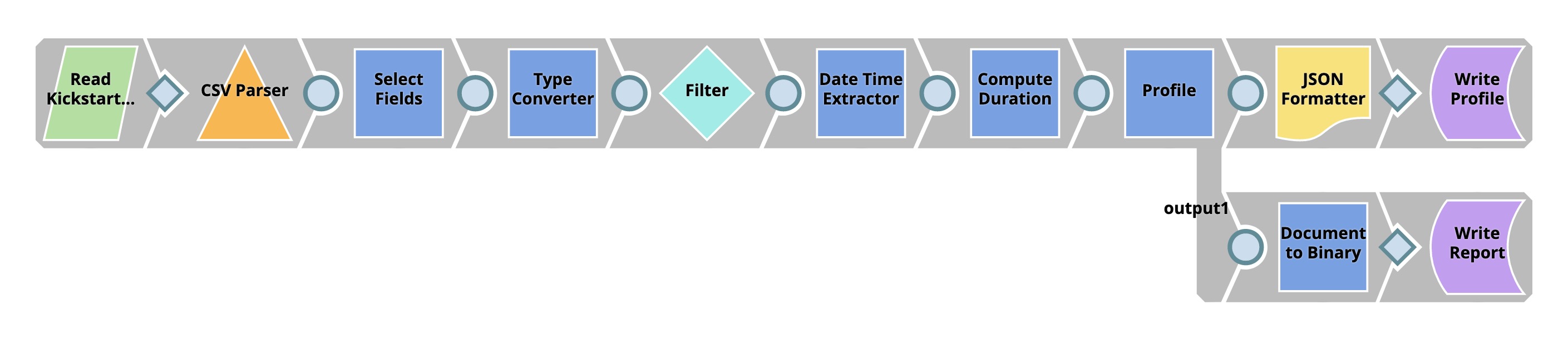
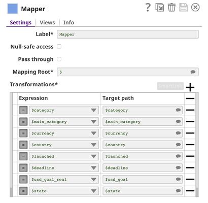
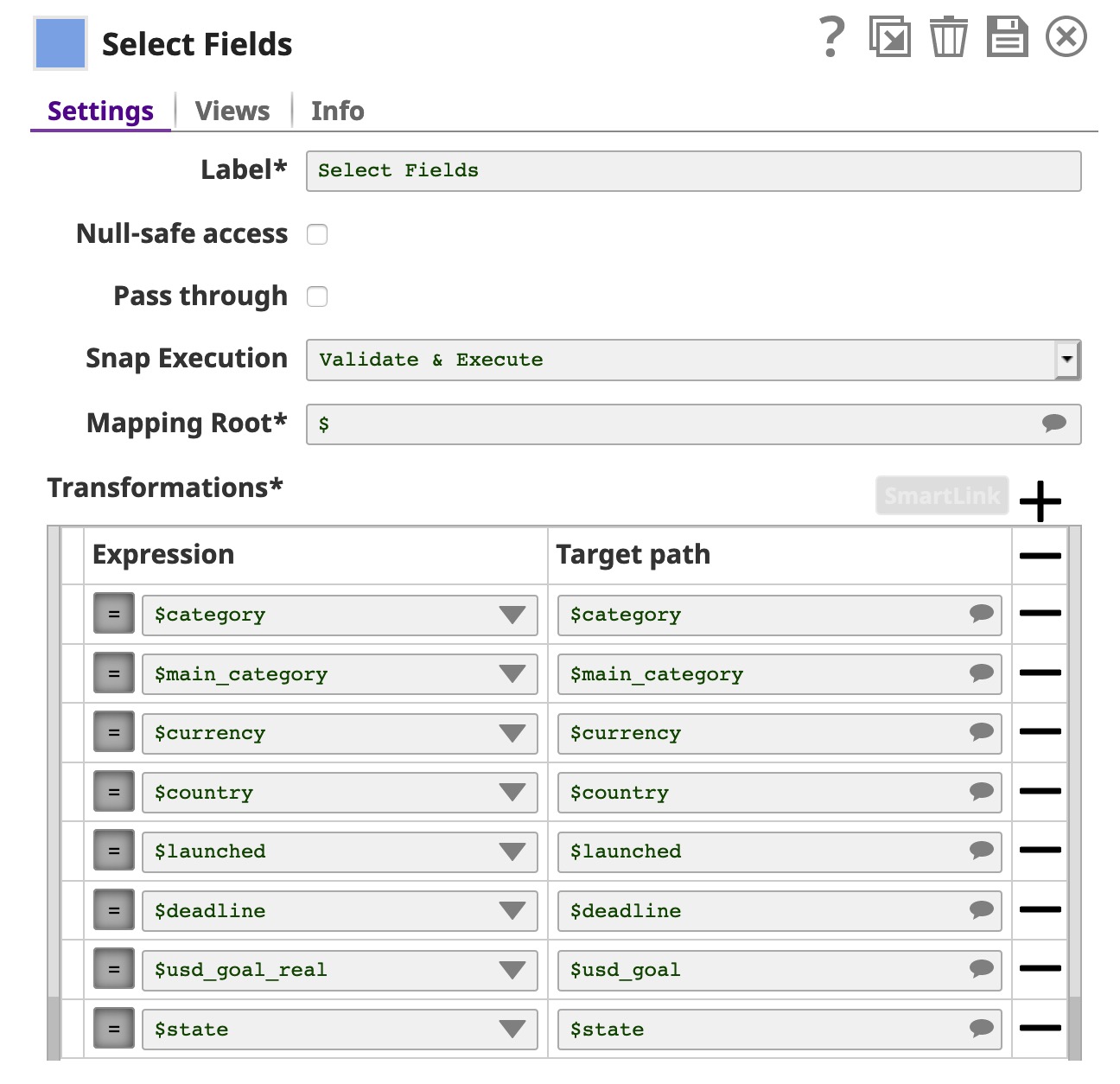
We use the first Mapper Snap (Select Fields) to select and rename fields.
Then, we use Type Converter Snap to automatically derive types of data.
...
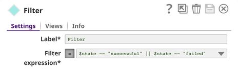
Since we only focus on successful and failed projects, we use Filter Snap to filter out live, canceled, and projects with another status.
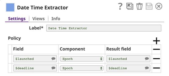
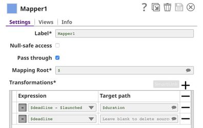
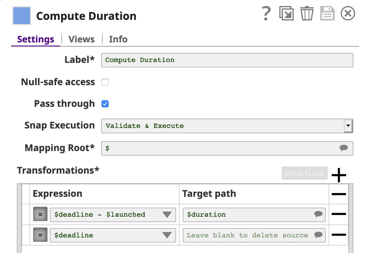
The Date Time Extractor Snap is used to convert the launch date and the deadline to an epoch which are used to compute the duration in the Mapper1 Mapper Snap (Compute Duration). With the Pass through in the Mapper1Mapper Snap, all input fields will be sent to the output view along with the $duration. However, we drop $deadline here.
At this point, the dataset is ready to be fed into the Profile Snap.
...
Finally, we use Profile Snap to compute statistics and save on SLFS in JSON format.
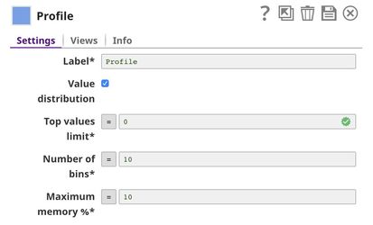
The Profile Snap has 2 output views. The first one is converted into JSON format and saved as a file. The second one is an interactive report which is shown below.
Click here to see the statistics generated by the Profile Snap in JSON format.
Data Preparation
In this pipelinePipeline, we want to transform the raw dataset into a format that is suitable for applying Machine Learning algorithms.
...
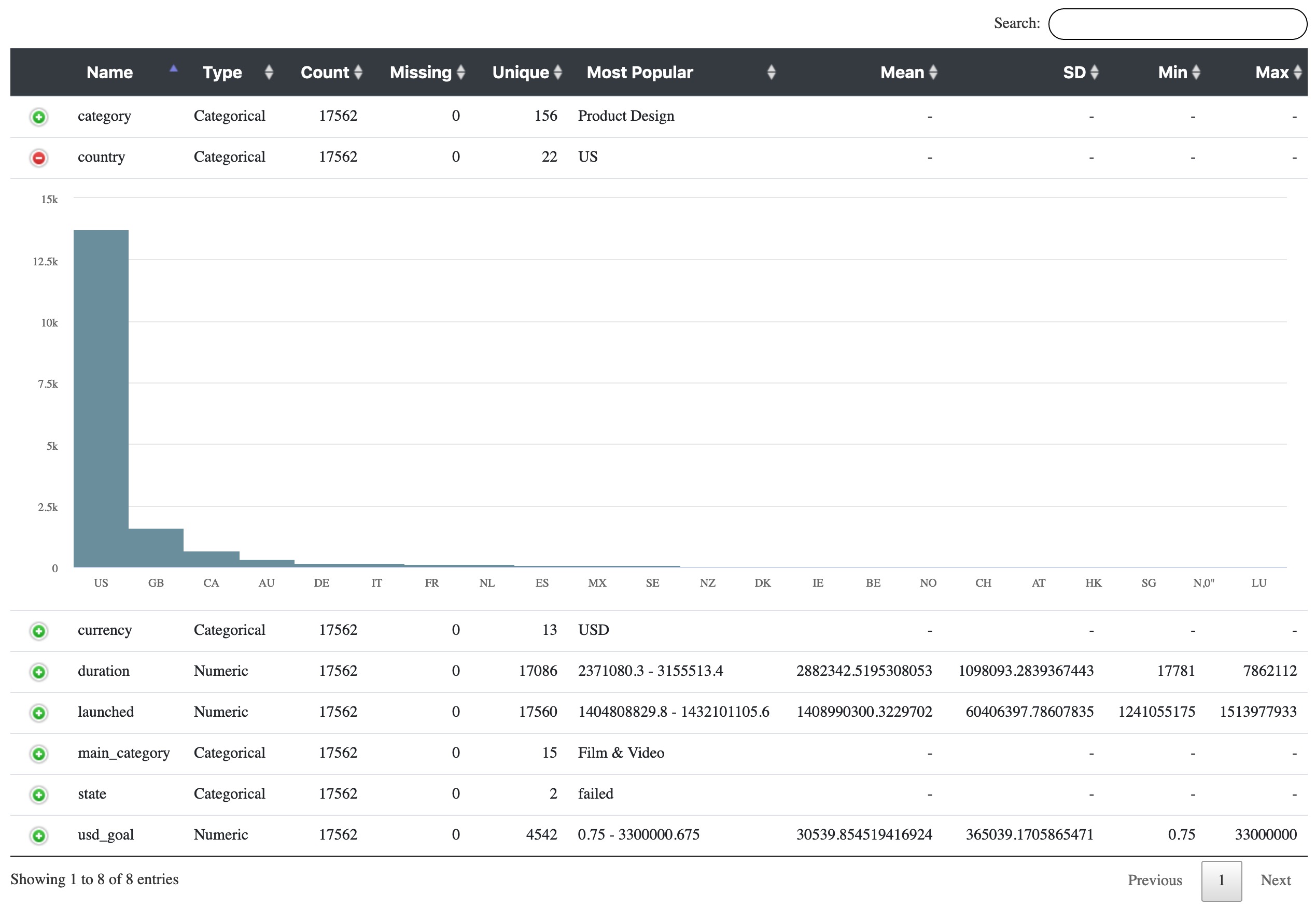
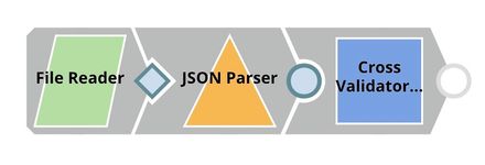
The first 7 Snaps in the top flow are the same as in the previous pipelinePipeline. We use File Reader1 Snap together with JSON Parser to read the profile (data statistics) generated in the previous pipelinePipeline. The picture below shows the output of JSON Parser Snap. Product design is the category with the most number of projects. USD is clearly the most popular currency. The country with the most number of projects is the USA.
...
Click here to see the statistics generated by the Profile Snap based on the processed dataset. As you can see, the min and max of all numeric fields are 0 and 1 because of the Scale Snap.
AutoML
This Pipeline builds several models within the resource limit specified in the AutoML Snap. There are 3 outputs: the model with the best performance, leaderboard, and report.
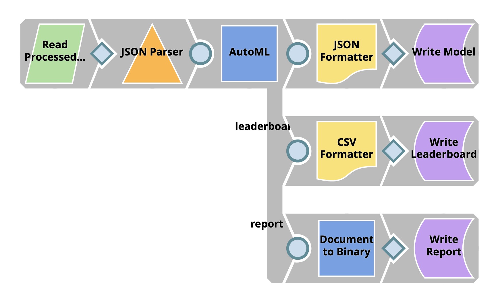
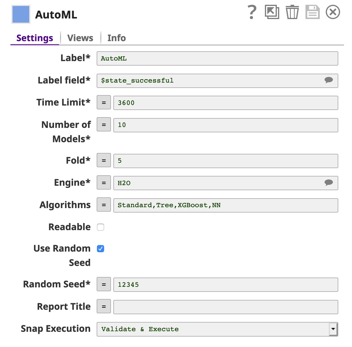
The File Reader Snap reads the processed data which we prepared using the Data Preparation Pipeline. Then, the AutoML Snap builds up to 10 models within the 3,600 seconds time limit. You can increase the number of models and time-limit based on the resources you have. You can also select the engine, this Snap supports Weka engine and H2O engine. Moreover, you can specify the algorithm you want this Snap to try.
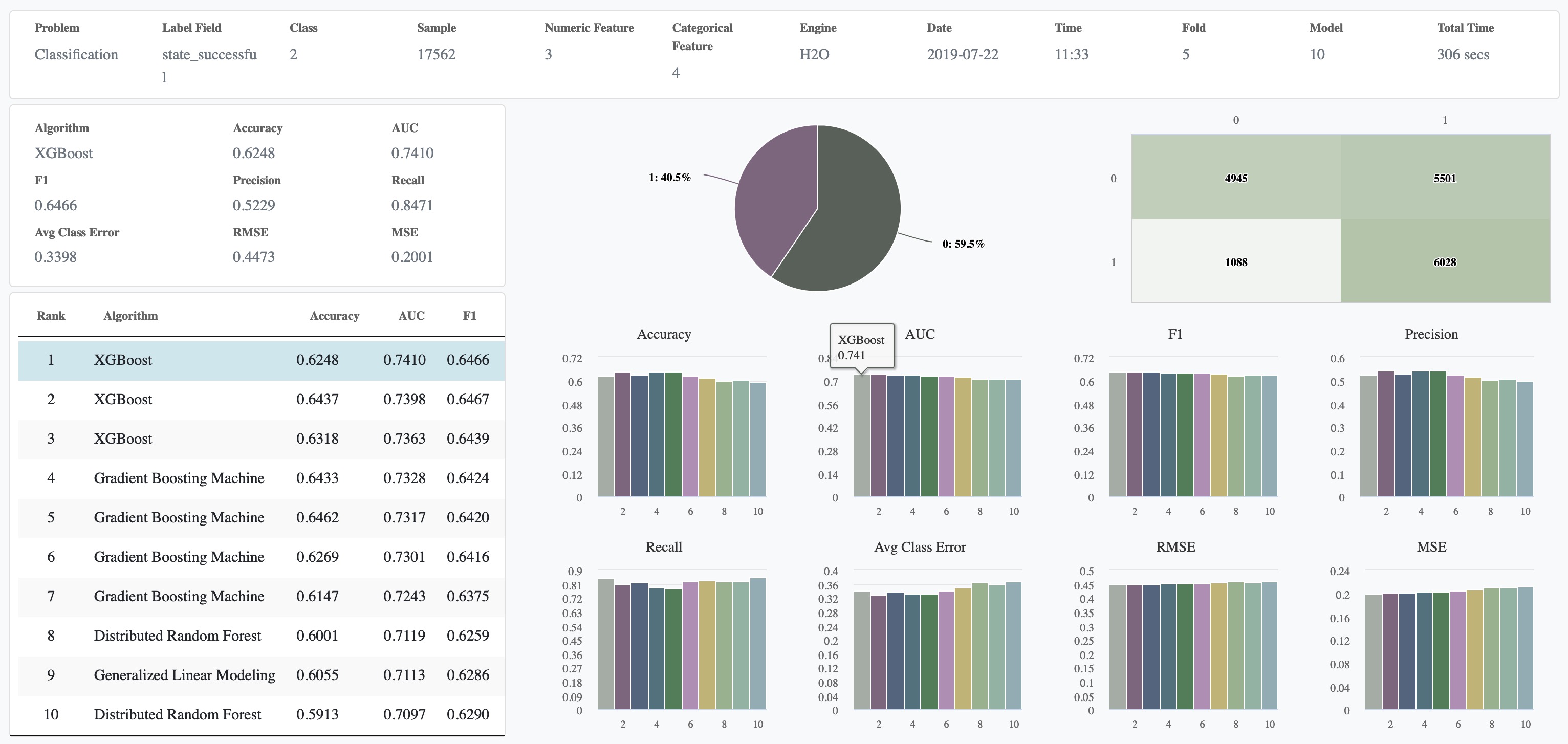
Below is the report from the third output view of the AutoML Snap. As you can see, the XGBoost model performs the best in this dataset with the AUC of 0.74.
Cross Validation
This pipeline Overall, the AutoML Snap is sufficient; however, if you prefer to specify the algorithm and parameters yourself, you can use the Cross Validator Snaps. This Pipeline performs 10-fold cross validation with various classification algorithms. Cross validation is a technique to evaluate how well a specific machine learning algorithm performs on a dataset. To keep things simple, we will use accuracy to indicate the quality of the predictions. The baseline accuracy is 50% because we have two possible labels: successful (1) and failed (0). However, based on the profile of our dataset, there are 7116 successful projects and 10446 failed projects. The baseline accuracy should be 10446 / (10446 + 7116) = 59.5% in case we predict that all projects will fail.
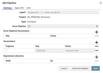
We have 2 pipelinesPipelines: parent and child. The parent pipeline Pipeline uses Pipeline Execute Snap to execute child pipeline Pipeline with different parameters. The parameter is the algorithm name which will be used by child pipeline Pipeline to perform 10-fold cross validation. The overall accuracy and other statistics will be sent back to the parent pipeline Pipeline which will write the results out to SLFS and also use Aggregate Snap to find the best accuracy.
...
The File Reader Snap reads the processed dataset generated by the data preparation pipeline Pipeline and feeds into the Cross Validator (Classification) Snap. The output of this pipeline Pipeline is sent to the parent pipelinePipeline.
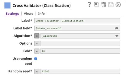
In Cross Validator (Classification) Snap, Label field is set to $state_successful which is the one we want to predict. Normally, you can select Algorithm from the list. However, we will automate trying multiple algorithms with Pipeline Execute Snap so we set the Algorithm to the pipeline Pipeline parameter.
Parent Pipeline
...
The $algorithm from CSV Generator will be passed into the child pipeline Pipeline as pipeline Pipeline parameter. For each algorithm, a child pipeline Pipeline instance will be spawned and executed. You can execute multiple child pipelines Pipelines at the same time by adjusting Pool Size. The output of the child pipeline Pipeline will be the output of this Snap. Moreover, the input document of the Pipeline Execute Snap will be added to the output as $original.
...
As you can see in the runtime below, 8 child pipeline Pipeline instances were created and executed. The 5th algorithm (Support Vector Machines) took over 17 hours to run. The last algorithm (Multilayer Perceptron) also took a long time. The rest of the algorithms can be completed within seconds or minutes. The duration depends on the number of factors. Some of them are the data type, number of unique values, and distribution.
...