On this Page
Problem Scenario
Customer churn is a big problem for service providers because losing customers results in losing revenue and could indicate service deficiencies. There are many reasons why customers decide to leave services. With data analytics and machine learning, we can identify the important factors of churning, create a retention plan, and predict which customers are likely to churn.
The live demo is available at our Machine Learning Showcase.
Dataset
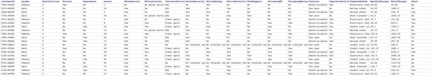
We use a dataset of telecommunication company which can be found here. This dataset contains 21 fields (columns). Each document (row) represents a customer record. We have data about customer's demographic, service subscriptions, and the field $Churn which indicates whether the customer has already left or not. There are 7043 customer records with 1869 churns. The following image shows a preview of this dataset:
Objectives
- Profiling: Use Profile Snap from ML Analytics Snap Pack to compute statistics of this dataset.
- Data Preparation: Perform data preparation on this dataset using Snaps from ML Data Preparation Snap Pack.
- Cross Validation: Use Cross Validator (Classification) Snap from ML Core Snap Pack to perform 10-fold cross validation on various Machine Learning algorithms. The result lets us know the accuracy of each algorithm in the churn prediction.
- Model Building: Use Trainer (Classification) Snap from ML Core Snap Pack to build the logistic regression model based on this dataset; then serialize and store.
- Model Hosting: Use Predictor (Classification) Snap from ML Core Snap Pack to host the model and build the API using Ultra Task.
- API Testing: Use REST Post Snap to send a sample request to the Ultra Task to make sure the API is working as expected.
- Visualization API: Use Remote Python Script Snap from ML Core Snap Pack to host API that can provide data visualization of the selected field in the dataset.
We are going to build 8 pipelines: one pipeline for each objective except for Cross Validation where we have 2 pipelines to automate the process of trying multiple algorithms. Each of these pipelines is described in the Pipelines section below.
Pipelines
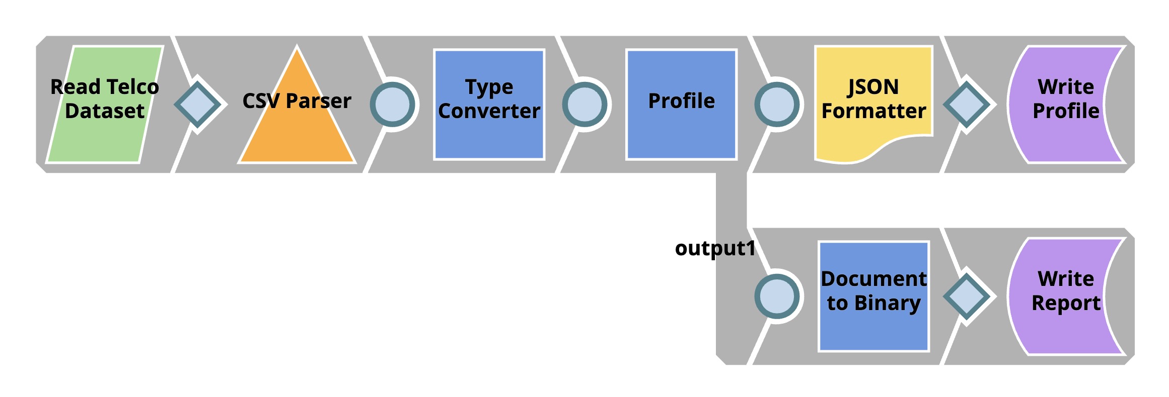
Profiling
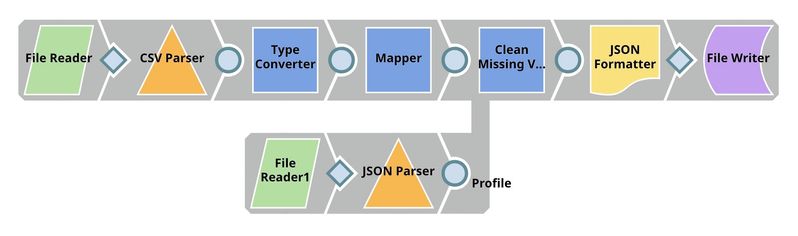
The File Reader Snap reads the dataset which is in CSV format. Then, the CSV Parser Snap parses the dataset into documents. In SnapLogic, there are two types of input/output view. The diamond shape is the binary view while the circle shape is the document view. Parser Snaps convert binary into document while Formatter Snaps convert document to binary.
In most cases, the output documents of CSV Parser Snap are represented as string data type even though some of them are supposed to be numeric. The Profile Snap gives different sets of statistics for numeric and categorical fields, so, we use the Type Converter Snap to automatically convert the data types. Then, we use JSON Formatter and File Writer Snaps to write the data statistics as a file on SnapLogic File System (SLFS). The Profile Snap also has a second output which is an interactive profile of the dataset. We use Document to Binary and File Writer Snaps to save the interactive profile in HTML format.
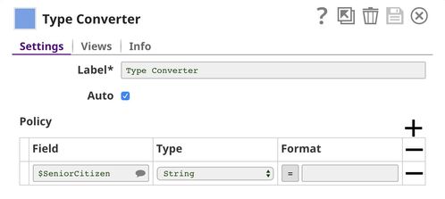
In this dataset, there is a field $SeniorCitizen which is categorical but contains 1 and 0 instead of Yes and No. The auto mode of the Type Converter Snap thinks that this field is numeric and converts those 0 and 1 into an integer. So, we need to add Policy that tells the Snap to convert values in $SeniorCitizen to string data type which represents categorical data.
Let's take a look at the data statistics computed by the Profile Snap.
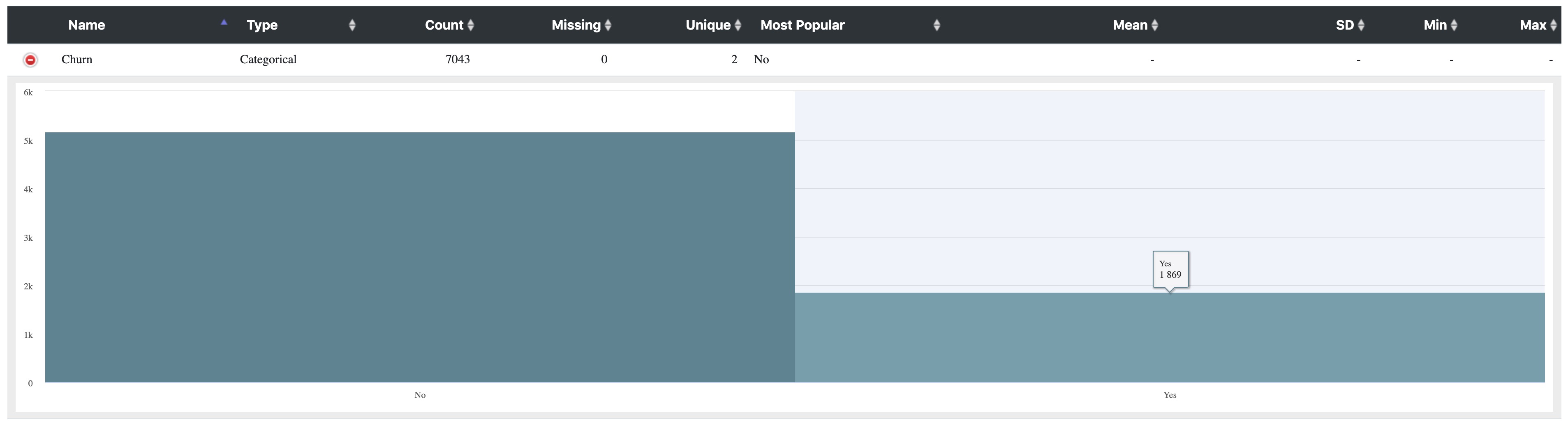
Below shows the profile of $Churn field. As you can see, 1869 of customers have already churned. There are 7043 - 1869 = 5174 who are stilling using the services.
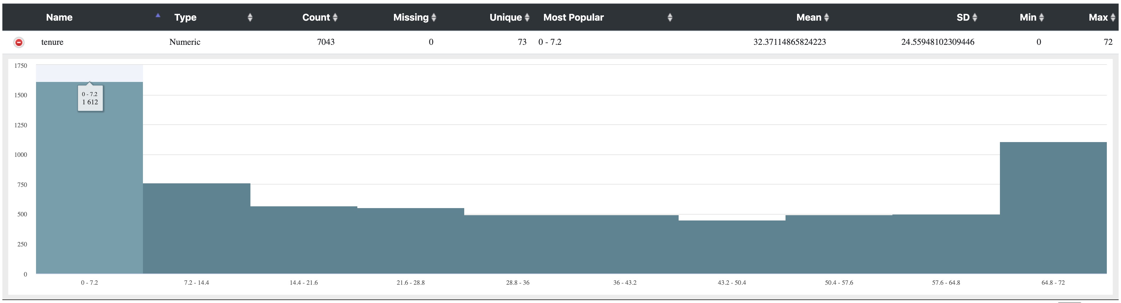
The picture below shows the histogram of $tenure field. There are 1612 customers (including churn) who use the services for less then 7.2 months. There are also large amount of customers who use the services for 64.8 - 73 months. The significant drops from 0 - 7.2 compared to 7.2 - 14.4 could indicate that customers churn a lot in the early stage.
Data Preparation
As mentioned in the previous pipeline section, $customerID field should be removed from the dataset and the missing values in $TotalCharges should be handled.
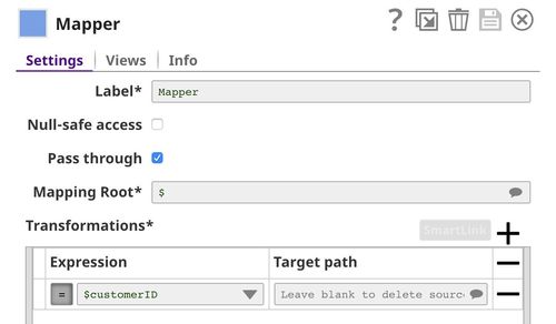
The Mapper Snap removes $customerID field from the input documents. In the Snap configuration, Pass through is selected to output all the fields. However, $customerID is removed according to the transformation we specify. Leaving the Target path property empty means removing the input field.
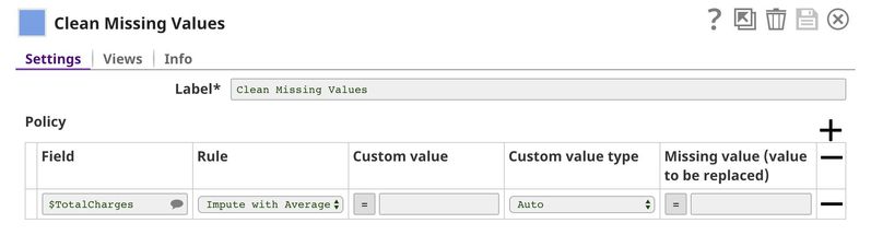
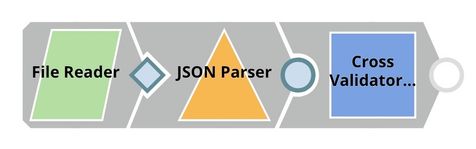
The Clean Missing Values Snap imputes missing values in $TotalCharges with the average value. When using Impute with Average, the data statistics are required. We use File Reader1 and JSON Parser Snaps to read the data statistics generated by the Profile Snap in the previous pipeline.
Cross Validation
In this step, we perform a 10-fold cross validation with various classification algorithms. Cross validation is a technique to evaluate how well a specific machine learning algorithm performs on a dataset. To keep things simple, we use accuracy to indicate the quality of the predictions. The baseline accuracy is 50% because we have two possible labels: churn and not churn. However, based on the data statistics of this dataset, there are 5174 customers who are not churning out of 7043 total customers. The baseline accuracy should be 5174 / 7043 = 73.5% in case we predict that all customers are not churning.
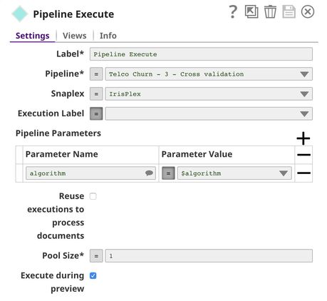
We have 2 pipelines: parent and child. The parent pipeline uses the Pipeline Execute Snap to execute the child pipeline with different parameters. The parameter is the algorithm name which will be used by the child pipeline to perform the 10-fold cross validation. The overall accuracy and other statistics will be sent back to the parent pipeline which will write the results to SLFS and also use the Aggregate Snap to find the best accuracy.
Child Pipeline
The File Reader Snap reads the processed dataset generated by the data preparation pipeline and feeds the dataset into the Cross Validator (Classification) Snap. The output of this pipeline is sent to the parent pipeline.
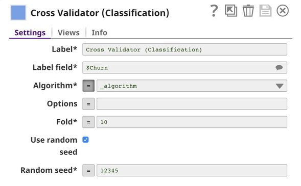
In the Cross Validator (Classification) Snap, Label field is set to $Churn which is the one we want to predict. Normally, you can select Algorithm from the suggested list. However, we will automate trying multiple algorithms with Pipeline Execute Snap so we set the Algorithm to the pipeline parameter. The default pipeline parameter can be set in the pipeline setting.
Parent Pipeline
This pipeline uses the Pipeline Execute Snap to execute the child pipeline multiple times with different classification algorithms. The goal is to find the algorithm that performs the best in this dataset.
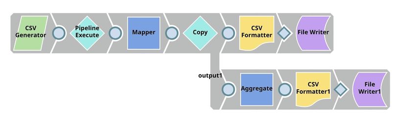
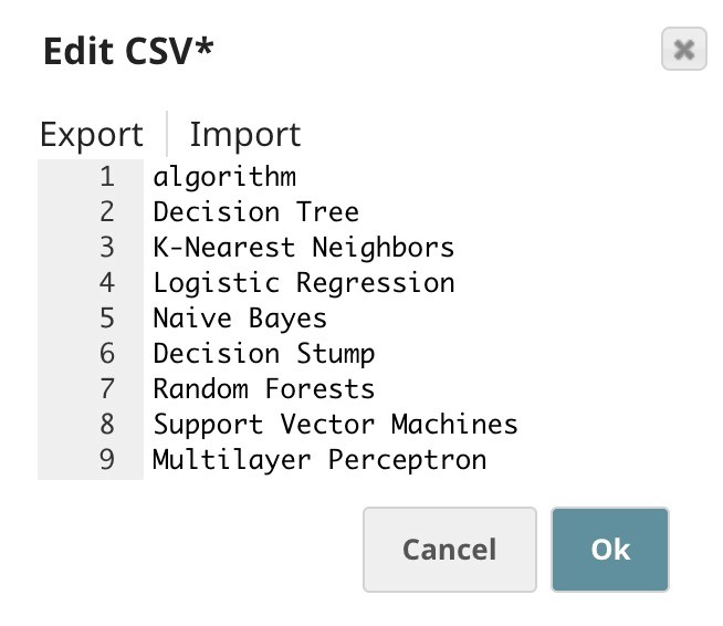
Below is the content of the CSV Generator Snap. It contains a list of algorithms we want to try.
The $algorithm from the CSV Generator Snap will be passed into the child pipeline as pipeline parameter. For each algorithm, a child pipeline instance will be spawned and executed. You can execute multiple child pipeline instances in parallel by adjusting Pool Size. The output of the child pipeline will be the output of this Snap. Moreover, the input document of the Pipeline Execute Snap will be added to the output as $original.
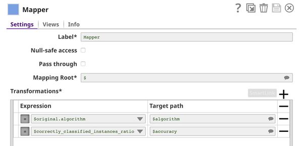
The Mapper Snap extracts the algorithm name and accuracy from the output of the Pipeline Execute Snap.
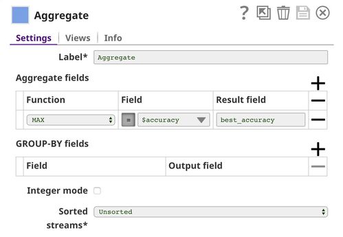
The Aggregate Snap finds the best accuracy among all algorithms.
As you can see in the runtime execution below, 8 child pipeline instances were created and executed. The 8th algorithm (Multilayer Perceptron) took almost 25 minutes to run. The rest of the algorithms can be completed within seconds or minutes. The duration depends on various factors; some of them are the data type, number of unique values, and distribution.
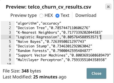
Following is the result. The logistic regression performs the best on this dataset at 80.6% accuracy. This is better than the baseline at 73.5%. However, it may not be practical to use. We may be able to do better than this by gathering more data about the customer or improving the algorithm.
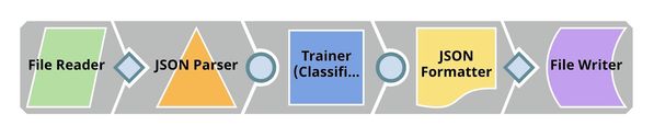
Model Building
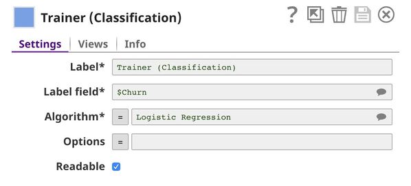
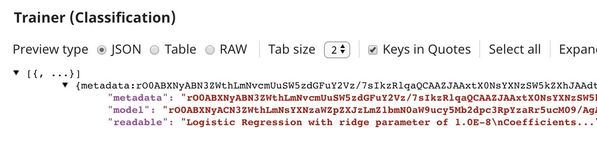
In this pipeline, we use the Trainer (Classification) Snap to build the model using logistic regression algorithm.
The File Reader Snap reads the dataset from Data Preparation pipeline which is in JSON Format. Then, the JSON Parser Snap converts binary data into documents. We do not need the Type Converter Snap since JSON file contains the data type. Then, the Trainer (Classification) Snap trains the model using logistic regression algorithm. The model consists of two parts: metadata describing the schema (field names and types) of the dataset, and the actual model. Both metadata and model are serialized. If the Readable property in the Trainer (Classification) Snap is selected, the readable model will be included in the output. Finally, the model is written as a JSON file to SLFS using JSON Formatter and File Writer Snaps.
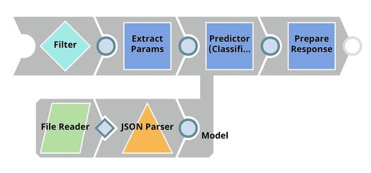
Model Hosting
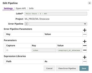
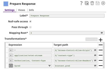
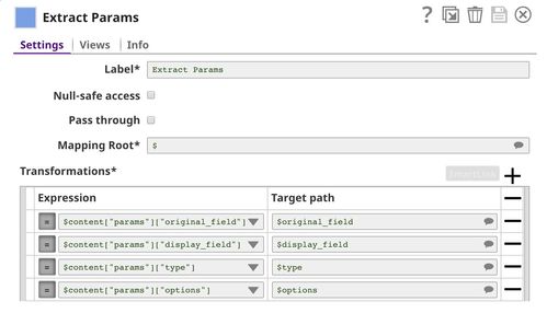
This pipeline is scheduled as an Ultra Task to provide a REST API that is accessible by external applications. The File Reader and JSON Parser Snaps read the model built by the previous pipeline. The Predictor (Classification) Snap takes the data from API requests and model from the JSON Parser Snap to give predictions. The Filter Snap authenticates the requests by checking the token that can be changed in the pipeline parameters. The Extract Params Snap (Mapper) extracts the required fields from the request. The Prepare Response Snap (Mapper) maps from prediction to $content.pred which will be the response body. This Snap also adds headers to allow Cross-Origin Resource Sharing (CORS).
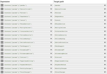
The following image on the left shows the expressions in the Extract Params Snap that extract required fields from the request. The image on the right shows the configuration of the Prepare Response Snap.
Building API
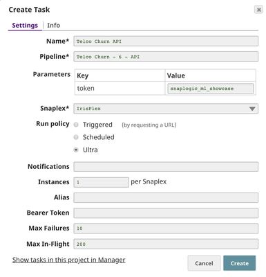
To deploy this pipeline as a REST API, click the calendar icon in the toolbar. Either Triggered Task or Ultra Task can be used.
Triggered Task is good for batch processing since it starts a new pipeline instance for each request. Ultra Task is good to provide REST API to external applications that require low latency. In this case, Ultra Task is preferable. Bearer token is not needed here since the Filter Snap will perform authentication inside the pipeline.
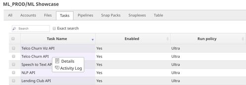
In order to get the URL, click Show tasks in this project in Manager in the Create Task window. Click the small triangle next to the task then Details. The task detail will show up with the URL.
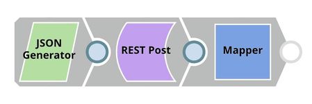
API Testing
In this pipeline, a sample request is generated by the JSON Generator. The request is sent to the Ultra Task by the REST Post Snap. The Mapper Snap extracts response which is in $response.entity.
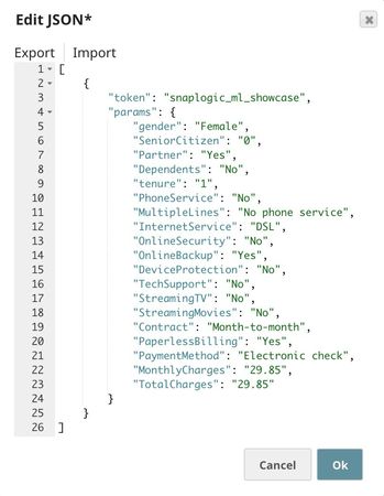
Below is the content of the JSON Generator Snap. It contains $token and $params which will be included in the request body sent by the REST Post Snap.
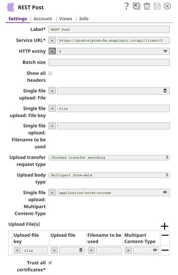
The REST Post Snap sends the request to the Ultra Task. Your URL can be found in the Manager page. In some cases, it is required to check Trust all certificates in the REST Post Snap.
The output of the REST Post Snap is shown below. The Mapper Snap extracts $response.entity from the response. In this case, the model predicts that this customer is likely to churn with the probability of 63.6%.

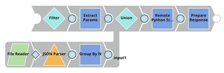
Visualization API
This pipeline reads the dataset using File Reader and JSON Parser Snaps. The Group By N Snap packs all documents (rows) in the dataset into one big document. Then, the dataset is buffered in the Remote Python Script Snap. When the request comes in, the Remote Python Script Snap draws a visualization and outputs as HTML which can be rendered in the UI. This pipeline is scheduled as an Ultra Task to provide an API to external applications. The instruction is the same as described in the previous section.
Below is the configuration of the Extract Params Snap. It extracts information from the request required by the Remote Python Script Snap to draw a visualization.
Python Script
Following is the script from the Remote Python Script Snap used in this pipeline. The script has the following 3 important functions:
- snaplogic_init
- snaplogic_process
- snaplogic_final
The first function (snaplogic_init) is executed before consuming the input data. The second function (snaplogic_process) is called on each of the incoming documents. The last function (snaplogic_final) is processed after all the incoming documents are consumed by snaplogic_process.
First, we use SLTool.ensure to automatically install the required libraries. SLTool class contains useful methods: ensure, execute, encode, decode, etc. In this case, we need bokeh which is the library we use to draw a visualization.
In snaplogic_process, the requests are buffered until the dataset is loaded. The dataset from the Group By N Snap is in row["group"]. Once the dataset is loaded, the requests can be processed. In this case, numeric and categorical fields will result in different types of visualization.
Downloads