Loan Repayment Prediction
- Kalpana Malladi
- Vidya Patil
- Anand Vedam
On this Page
Problem Scenario
LendingClub provides peer-to-peer lending services. Someone who wants to invest can open an investor account, or someone who requires money can avail a loan. The platform lends money from investors to borrowers. LendingClub has been operating since 2007 and over 1.5M loans have been approved so far.
Approving a loan is challenging. Firstly, a loan can either be approved or rejected. Then, the approved loan can end up being fully paid or charged off. A strict policy would reduce the charged off rate but would also mean a lesser number of loan approvals. This issue is not only for LendingClub but applies to all financial institutes.
In this use case, we want to build a machine learning model that can identify loans that are likely to end up being charged off. If we succeed, we will be able to reduce the loss from charged off loans and use that money to invest in something else.
The live demo is available at our Machine Learning Showcase.
Check the Profit Analysis section to see how much money we can save with machine learning.
Dataset
There are 2 datasets in this model: approved loans and rejected loans. You can download the datasets from here. In this use case, we focus only on the approved loans and only include fully paid and charged off loans. This dataset contains 646902 fully paid loans and 168084 charged off loans since 2007. Since the term of a loan can be either 36 or 60 months, we have used loans approved until 2014 as a training set, and loans approved in 2015 as a test set. Most of the loans approved after 2015 are in progress and we do not know whether they will be fully paid or charged off, and hence, they are excluded.
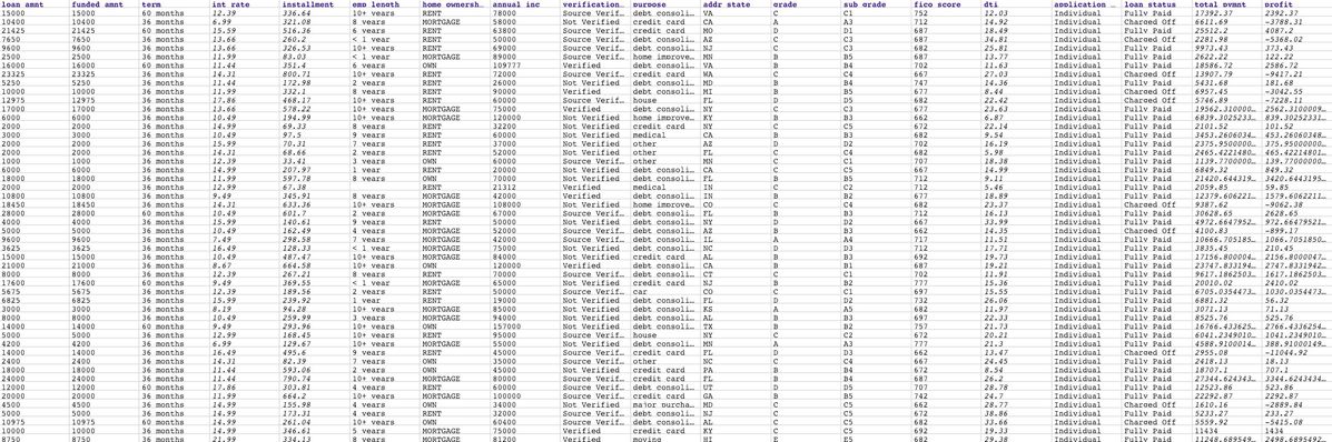
The following image shows the preview of the test set. The training set is in the same format except that it does not contain $total_pymnt and $profit. To keep things simple, we compute the profit by subtracting $funded_amnt from $total_pymnt. Those two are used in the profit analysis. The training set and test set can be found here.
Process Summary
| Pipeline | Description |
|---|---|
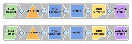
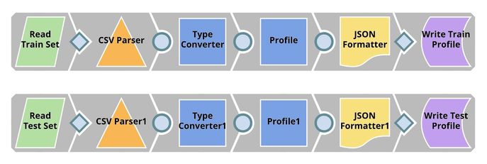
| Profiling. This pipeline reads the training set and test set from GitHub, performs type conversion, and computes data statistics which is saved to SnapLogic File System (SLFS) in a JSON format. |
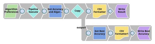
| Cross Validation. We have 2 pipelines in this step. The first pipeline (child pipeline) performs k-fold cross validation using a specific ML algorithm. The second pipeline (parent pipeline) uses Pipeline Execute Snap to automate the process of performing k-fold cross validation on multiple algorithms. The Pipeline Execute Snap spawns and executes child pipeline multiple times with different algorithms. Instances of child pipeline can be executed sequentially or in parallel to speed up the process by taking advantage of multi-core processor. The Aggregate Snap applies max function to find the algorithm with the best result. |
| |
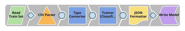
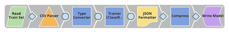
| Model Building. Based on the cross validation result, there is no best algorithm on this dataset. Most of them perform at the same level. Trainer (Classification) Snap trains Random Forests model which is formatted to JSON and compressed. The compressed JSON is written to SLFS. |
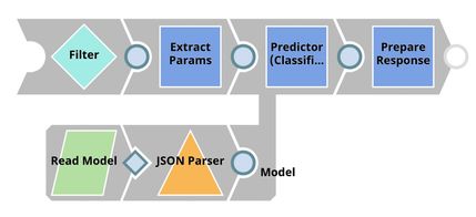
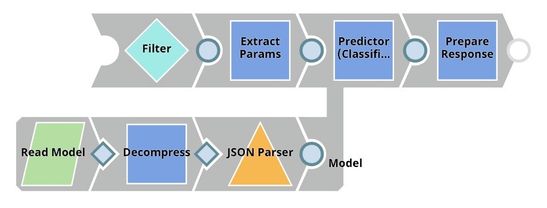
| Model Hosting. This pipeline is scheduled as an Ultra Task to provide REST API to external applications. The request comes into an open input view. The core Snap in this pipeline is Predictor (Classification) which hosts the ML model from JSON Parser Snap. Filter Snap drops the requests with an invalid token. Extract Params (Mapper) Snap extracts input from the request. See more information here. |
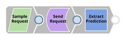
| API Testing. JSON Generator Snap contains a sample request including token and text. REST Post Snap sends a request to the Ultra Task (API). Mapper Snap extracts prediction from the response body. See more information here. |
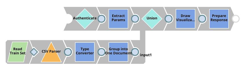
| Visualization API. This pipeline is scheduled as an Ultra Task to provide REST API to external applications. Remote Python Script Snap stores the dataset (from the bottom flow) in memory and generates visualization for each incoming request from the top flow. Filter Snap drops the requests with an invalid token. Extract Params (Mapper) Snap extracts input from the request. See more information here. |
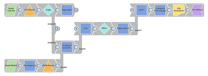
| Profit Analysis. This pipeline uses the trained model to predict the charged-off rate of loans in the test set. The Filter Snap rejects some of the loans based on the confidence level. The Aggregate Snaps compute statistics (before and after applying the ML model) including the number of approved loans, total fund, total profit, and average profit per loan. Finally, Mapper Snap computes the percentage of improvement. |


Key Snaps
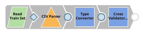
Profiling
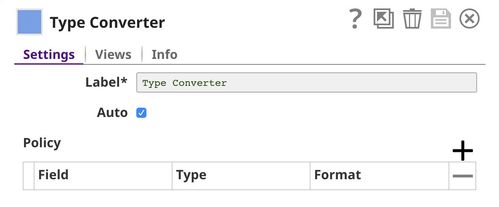
Type Converter
File Reader (Read Train / Test Set) Snaps read the datasets which are in CSV format. CSV file does not maintain the data type so the CSV Parser Snap will output data as text represented by String data type. This dataset contains 7 numeric fields (with additional two fields in the test set): loan_amnt, funded_amnt, int_rate, installment, annual_inc, fico_score, and dti. Hence, we need to use the Type Converter Snap to convert them. The output contains the dataset which looks similar to the output of the CSV Parser Snap. However, the numeric fields are now represented as BigInteger and BigDecimal data types.
Profile
This Snap computes data statistics of the dataset. You can see the output of this Snap for training set here and for the test set here.
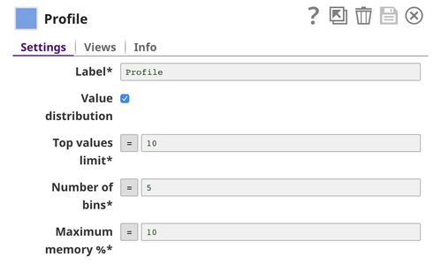
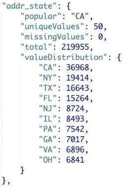
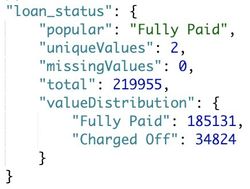
The output contains data statistics of this dataset. The following images show the profile of $addr_state and $loan_status in the training set. As you can see, California state has the most loans.
There are 185131 (84.17%) fully paid loans and 34824 (15.83%) charged-off loans.
Cross Validation
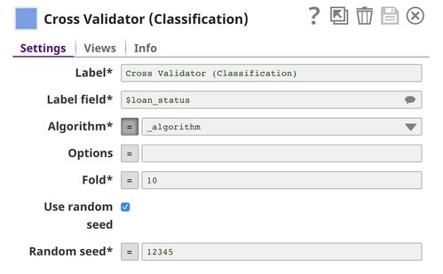
Cross Validator (Classification)
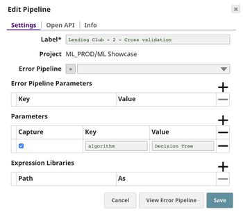
This Snap performs 10-fold cross validation using the algorithm specified by _algorithm which is a pipeline parameter passed into this pipeline by the Pipeline Execute Snap in the parent pipeline. You can set the default values for pipeline parameters in the pipeline settings.
The output contains statistics of the cross validation result. $correctly_classified_instances_ratio is the accuracy.
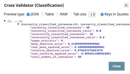
This is the result of the pipeline validation based on the first 50 documents in the dataset. The result based on the full dataset is generated when the pipeline is executed.
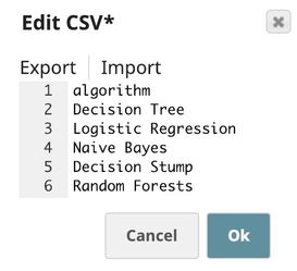
CSV Generator
This Snap contains a list of algorithms we want to try. In this case, we specify 5 algorithms. You may try Support Vector Machines or Multilayer Perceptron which will take a longer time to complete.
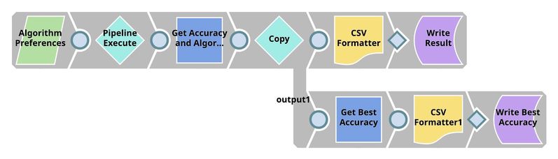
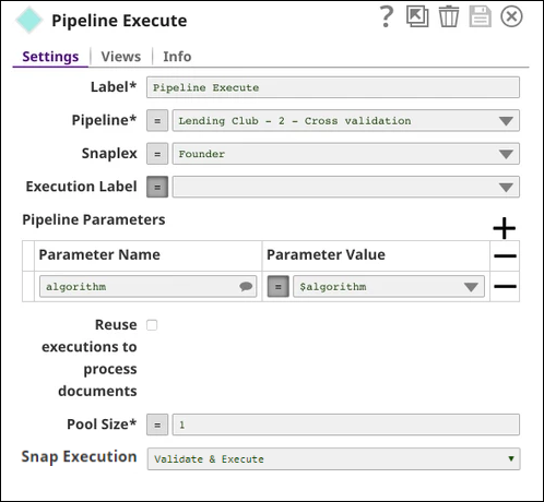
Pipeline Execute
This Snap spawns and executes the child pipeline (Lending Club - 2 - Cross validation) 5 times, each time with a different algorithm as specified by $algorithm from the CSV Generator Snap. You can specify the Pool Size to be greater than 1 to execute multiple child pipeline instances in parallel.
The output contains statistics of the cross validation results from the child pipeline executions. The $original includes the input of the Pipeline Execute Snap. In this case, it contains $algorithm from the CSV Generator Snap.
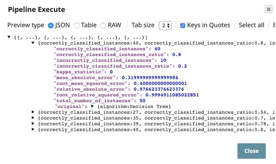
This is the result of the pipeline validation based on the first 50 documents in the dataset. The result based on the full dataset will be generated when the pipeline is executed.
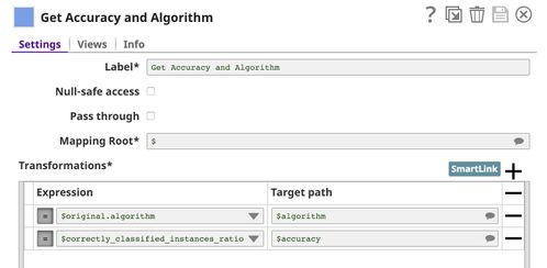
Mapper
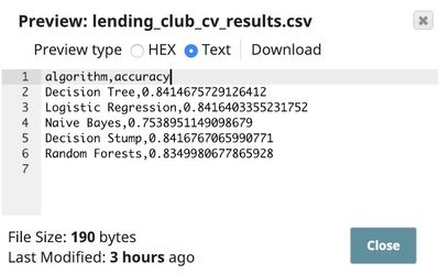
This Snap outputs the algorithm name together with the accuracy which is defined as $correctly_classified_instances_ratio. The rest of the statistics are removed. You can change this to the metric of your choice.
The output contains the algorithm name together with the accuracy. We use CSV Formatter and File Writer Snaps to write the results to the SnapLogic File System (SLFS) in CSV format. As you can see, decision tree, logistic regression, and decision stump perform at about 84% accuracy. We know that this training set contains 84.17% of fully paid loans. So, it could be that the ML algorithms are biased towards "fully paid" and rarely predict "charged off". Accuracy is not a good metric in this case. Random forests algorithm seems to try harder in predicting "charged off" even though it has slightly lower accuracy.
However, our goal is to reduce the loss and maximize the profit, we will compute the profit improvement based on the test set and apply threshold adjustment in Profit Analysis section. According to the profit analysis, logistic regression and random forests perform the best. In the next section, we will build the random forests model and host it as an API.
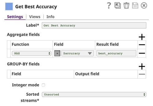
Aggregate
This Snap applies max function to find the best accuracy.
Model Building
Trainer (Classification)
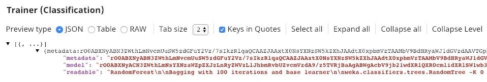
This Snap trains the ML model using the random forests algorithm. You can see all the available algorithms with their options here.
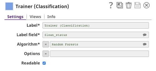
The output contains $metadata and $model which are serialized. Since we select Readable in the Trainer (Classification) Snap, the output includes the model in a readable format. You can use Mapper, Document to Binary, and File Writer Snaps to extract $readable and write it out as a text file. Compress Snap is optional, it helps reduce the size of the model file.
This is the result of the pipeline validation based on the first 50 documents in the dataset. The result based on the full dataset will be generated when the pipeline is executed.
Model Hosting
Follow the instructions here to schedule this pipeline as REST API.
Predictor (Classification)
This Snap hosts the model from the JSON Parser Snap and gives a prediction to each request coming from Extract Params (Mapper) Snap. If the Confidence level is selected, the predictions include the confidence level ranging from 0 to 1.

lending_club-5-predictor_snap.jpg
API Testing
You can find more information about API testing here.

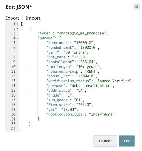
JSON Generator
This Snap contains a sample request which is sent to the API by the REST Post Snap.
Visualization API
Remote Python Script
This Snap loads the dataset from the Group By N Snap into the memory and gives a visualization based on the incoming requests from the Extract Params (Mapper) Snap. We use bokeh to draw visualization. To use Remote Python Script Snap, you must have Remote Python Executor installed on the Snaplex.
Profit Analysis
The test set includes 208143 loans approved in 2015. There are 169973 fully paid loans and 38170 charged off loans. To keep things simple, we compute the profit of loans based on $total_pymnt - $funded_amnt. It is possible that we make some profit from charged off loans. However, most of the charged off loans result in a loss (negative profit).
This section includes the profit analysis in multiple cases: without ML, decision tree, logistic regression, naive bayes, decision stump, random forests, and AutoML.
Without ML
The table below shows the statistics of the loans in the test set before applying the ML model.
| Title | Value |
|---|---|
| Approved Loan | 208,143 |
| Total Fund | $2,961,163,300 |
| Total Profit | $188,794,190.1 |
| Average Profit per Loan | $907.0408 |
With ML
The table below shows the statistics of the loans after applying various ML models with a default threshold (t=0.5). As you can see, the decision tree model always predicts "Fully Paid" and 0 loan is rejected. For logistic regression, only 0.46% of loans have been rejected and we get 1.12% more profit with 0.58% less fund. Random forests model rejects more loans than logistic regression which brings down the fund but earns less profit. AutoML seems to perform the best with 4% profit improvement with 2.47% less fund.
| Title | Decision Tree | Logistic Regression | Naive Bayes | Decision Stump | Random Forests | AutoML (90 Minutes + 20 Models) |
|---|---|---|---|---|---|---|
| Approved Loan | 0% | -0.47% | -24.00% | -0.001% | -2.22% | -1.90% |
| Total Fund | 0% | -0.58% | -31.97% | -0.0008% | -2.79% | -2.47% |
| Total Profit | 0% | +1.12% | -10.56% | +0.006% | +0.52% | +4.00% |
| Average Profit per Loan | 0% | +1.59% | +17.68% | +0.007% | +2.80% | +6.02% |
Threshold Adjustment
In general, ML algorithms optimize the metric based on the default threshold which is 0.5 for binary classification. In many cases, adjusting the threshold significantly improves the model. The following table shows the profit analysis with different threshold values ranging from 0.5 (default) to 0.8. If we focus on the profit, t=0.7 is the best. If you focus on minimizing the fund, t=0.8 may be a better option.
The best practice would be separating the data into 3 sets: training, validation, and test. Train the model based on the training set. Apply threshold adjustment based on the validation set. And evaluate the model using the test set.
| Title | AutoML (90 Minutes + 20 Models) | AutoML with t=0.6 | AutoML with t=0.7 | AutoML with t=0.8 |
|---|---|---|---|---|
| Approved Loan | -1.90% | -4.91% | -10.58% | -23.86% |
| Total Fund | -2.47% | -6.47% | -13.89% | -28.49% |
| Total Profit | +4.00% | +7.99% | +9.05% | -1.42% |
| Average Profit per Loan | +6.02% | +13.57% | +21.96% | +29.48% |
Downloads
Have feedback? Email documentation@snaplogic.com | Ask a question in the SnapLogic Community
© 2017-2025 SnapLogic, Inc.